Google Summer of Code 2016
Looking back at the eventful summer!
This project is maintained by mronian

Before the Coding Period | Summary of Contributions | Exposure Correction | Feature Extraction | Drawing on Images | Miscelleanous | Future Work
Whew. What an amazing summer it has been! It seems like just yesterday that I found myself among the lucky students who were selected for GSoC 2016. To make the news even more amazing, along with me 14 other students had been selected from my college! The efforts of previous GSoC alumni like Harsh and Abhishek to spread the culture of open source programming seemed to have paid off as this was a far cry from earlier years when only a handful of people used to participate. I can't thank both of them enough for helping me draft my proposal and giving valuable suggestions.
My proposal for this summer was to work on ImageFeatures.jl, a new Julia package for Feature Extraction and Descriptors in Images. Alongside this, I planned to add Exposure Correction functionality to Images.jl, an existing package for Image Processing in Julia.
One of the fun moments of the summer was getting a chance to attend JuliaCon 2016 at MIT, Boston! The Julia Language had generously invited all GSoCers to come and present their projects. My talk can be viewed below. Although I messed up the slides a bit and wasn't prepared for the talk, overall I guess it wasn't too shabby ;)
As we reach the final week of GSoC, it feels great to have managed to achieve most of my goals for the summer and gotten the chance to work with amazing people in the JuliaImages organisation as we attempt to develop a full fledged Computer Vision library of which ImageFeatures.jl is an essential part. I hope to continue to work and contribute more packages above and beyond GSoC as we slowly build up the organisation.
I would like to thank my mentors Tim Holy and Simon Danisch for helping me out throughout the summer and guiding me towards achieving my goals. Their friendliness and approachability made the summer a enjoyable and fruitful experience.
Before the Coding Period
TestImages.jl
In the initial phase of drafting my proposal, I had played around with Images.jl and TestImages.jl to understand the packages and try to make some initial contributions to the same. In the process, I felt that TestImages.jl needed a proper documentation along with a guide for contributing test images. Apart from the documentation, there was also a need to store the test images in a proper repository so that the links would not expire. Once my proposal was selected, I started working on this and with help from Tim Holy, I developed a new website for TestImages.jl along with an improved API to easily download images from the repository. The new API checks if the requested image is present in the online repository if it is not found locally and downloads it for the user.
The documentation can be viewed here.
Histograms
To get familiar with open source and Images.jl, one of my first PRs was to add the histogram functionality. This was a very simple function which would calculate the histogram of an image i.e. the intensity distribution.
edges, count = imhist(img, nbins)
edges, count = imhist(img, nbins, minval, maxval)
This generates a histogram for the image over nbins spread between (minval, maxval]. If minval and maxval are not given, then the minimum and maximum values present in the image are taken. edges specifies the range of the bins while count is a vector of the individual counts of the bins.
Summary of Contributions
| Package | Merged Commits | Pull Requests (Open and Merged) |
|---|---|---|
| Images.jl | Link | Link |
| ImageFeatures.jl | Link | Link |
| ImageDraw.jl | Link | Link |
| TestImages.jl | Link | Link |
| ColorVectorSpace.jl | Link | Link |
| ColorTypes.jl | Link | Link |
Exposure Correction
The first part of my proposal was to add exposure correction functionality to Images.jl. This was a bit challenging considering the various type of Images and ColorTypes in julia and my goal was to provide a common API which would handle all types of Images using julia's method dispatch. I am happy to say that we were able to do this to a considerable extent and all the functions are easy to use and intuitive, offering a lot of options at the same time.
Histogram Equalisation
My first contribution during the coding period was the histogram equalisation functionality. This took up quite a bit of time as I worked on optimising the performance and got to learn about the inner workings of Arrays (Images are derived from Arrays!) in julia and how to write efficient functions for operating on them. I was also introduced to @code_warntype and how to julia infers the type of variables in the code and how to best exploit this to increase performance. Tim Holy was really helpful and patient (Thanks Tim!) throughout the initial phase with a lot of code reviews and advice which really helped me later on.
hist_equalised_img = histeq(img, nbins)
hist_equalised_img = histeq(img, nbins, minval, maxval)
This returns a histogram equalised image with a granularity of approximately nbins number of bins. If minval and maxval are specified then intensities are equalized to the range (minval, maxval). The default values are 0 and 1.
Histogram Matching
Histogram matching is another way of achieving exposure correction by trying to modify the histogram of the image to match that of a predefined image with the desired histogram.
hist_matched_img = histmatch(img, oimg, nbins)This returns a grayscale histogram matched image with a granularity of nbins number of bins. img is the image to be matched and oimg is the image having the desired histogram to be matched to.
Gamma Correction
Gamma correction is a method of enhancing or reducing the intensity levels in an image by using a power function.
gamma_corrected_img = adjust_gamma(img, gamma)The adjust_gamma function can handle a variety of input types. The returned image depends on the input type. If the input is an Image then the resulting image is of the same type and has the same properties.
Contrast Limited Adaptive Histogram Equalisation
An advanced version of histogram equalisation, it differs from ordinary histogram equalization in the respect that the adaptive method computes several histograms, each corresponding to a distinct section of the image, and uses them to redistribute the lightness values of the image. It is therefore suitable for improving the local contrast and enhancing the definitions of edges in each region of an image.
In the straightforward form, CLAHE is done by calculation a histogram of a window around each pixel and using the transformation function of the equalised histogram to rescale the pixel. Since this is computationally expensive, we use interpolation which gives a significant rise in efficiency without compromising the result. The image is divided into a grid and equalised histograms are calculated for each block. Then, each pixel is interpolated using the closest histograms.
hist_equalised_img = clahe(img, nbins, xblocks = 8, yblocks = 8, clip = 3)The xblocks and yblocks specify the number of blocks to divide the input image into in each direction. nbins specifies the granularity of histogram calculation of each local region. clip specifies the value at which the histogram is clipped. The excess in the histogram bins with value exceeding clip is redistributed among the other bins.
Feature Extraction
After working on exposure correction, I began with the other major chunk of my proposal which was ImageFeatures.jl. Edge and corner detection was already a part of Images.jl so I added some of my work in the same to Images.jl itself (this will be moved to ImageFeatures.jl before release).
Canny Edge Detection
The canny edge detector works by finding intensity gradients of an image and then double thresholding pixels as being part of weak or strong edges. Then the weak edges not connected to any strong edge are discarded and the result has the edges detected in the image.
canny_edges = canny(img, sigma = 1.4, upperThreshold = 0.80, lowerThreshold = 0.20)Results of using the Canny edge detector on an image.

Corner Detection
I worked on the imcorner API to overhaul the existing corner detection functions and added additional functionality with
kitchen_rosenfeld corners and FAST corners (discussed below).
corners = imcorner(img; [method])
corners = imcorner(img, threshold, percentile; [method])
The method argument takes in the name of the algorithm to be used to detect corners, namely harris, shi_tomasi and kitchen_rosenfeld.
FAST Corners
FAST (Features from Accelerated Segment Test) corners, an efficient and very popular corner detection algorithm works by finding a contiguous set of pixels brighter or darker than the candidate pixel. Depending on the number of contiguous pixels found, the candidate is marked as a potential corner.
FAST corners may be detected by using the fastcorners API.
corners = fastcorners(img, n, threshold)Results of using the FAST Corner detector on an image.

ImageFeatures.jl
I started work on ImageFeatures.jl by adding texture matching descriptors like GLCMs (Gray Level Co-occurence Matrix) and LBPs (Local Binary Patterns).
Gray Level Co Occurence Matrices
Gray Level Co-occurrence Matrix (GLCM) is used for texture analysis. We consider two pixels at a time, called the reference and the neighbour pixel. We define a particular spatial relationship between the reference and neighbour pixel before calculating the GLCM.
The GLCM is calculated by calling one of glcm, glcm_symmetric or glcm_norm functions depending on the desired GLCM type.
glcm = glcm(img, distance, angle, mat_size)If multiple GLCMs need to be calculated, the same function may be used by passing a vector in the arguments. The distance and angle arguments take in both Int and Vector{Int} values.
Multiple properties of the obtained GLCM can be calculated by using the glcm_prof function which calculates the property of the entire matrix or in windows if given the window dimensions.
prop = glcm_prop(glcm, property)
prop = glcm_prop(glcm, height, width, property)
Various properties can be calculated like mean, variance, correlation, contrast, IDM (Inverse Difference Moment), ASM (Angular Second Moment), entropy, max_prob (Max Probability), energy and dissimilarity.
Local Binary Patterns
Local Binary Pattern (LBP) is a very efficient texture operator which labels the pixels of an image by thresholding the neighborhood of each pixel and considers the result as a binary number. The feature vector can now then be processed using some machine-learning algorithm to classify images. Such classifiers are often used for face recognition or texture analysis.
We have multiple type of LBP algorithms in ImageFeatures.jl :
The first three methods can be used with both circular offsets (circle around the pixel) or the 8x8 neighbourhood.
The first two methods, lbp and modified_lbp may be called with one of three lbp_original, lbp_uniform and lbp_rotation_invariant as the method argument which specifies the method used to create the bit pattern.
-
lbpis the original algorithm defined in the `94 paper. -
modified_lbpis a version of LBP which compares the intensity of each pixel with the average intensity in the window. -
direction_coded_lbpis a version of LBP where the intensity differences along the four directions (N-S, NW-SE, NE-SW, E-W) are coded along with the variation in differences along the directions in 8 bits. -
multi_block_lbpis a version of LBP used for window matching as an alternative to Haar like features. The image is divided into blocks and the average intensity of each block is considered with the center block to obtain the LBP.
lbp_image = lbp(img)
lbp_image = lbp(img, 10, 2) # With circular offsets
lbp_image = lbp(img_gray, lbp_uniform)
lbp_image = lbp(img_gray, lbp_rotation_invariant)


lbp_image = modified_lbp(img_gray)
lbp_image = modified_lbp(img_gray, points, radius)

lbp_image = direction_coded_lbp(img)
lbp_image = direction_coded_lbp(img, points, radius)

pattern = multi_block_lbp(img, top_left_y, top_left_x, height_block, width_block)
We can also create the descriptor from a histogram of LBPs over the image by calling create_descriptor.
desc = create_descriptor(img, yblocks, xblocks, [lbp_type])The lbp_type argument takes in one of the functions defined above, while the yblocks and xblocks arguments specify the size of the grid to create in the image.
Framework
Before starting with the feature descriptors, we decided on a easy to use common API which could be used with all the algorithms.
The Feature and Keypoint types are the fundamental types in ImageFeatures.jl. Feature stores the keypoint and its orientation and scale. A vector of the Feature type is denoted by the Features type and similary a vector of Keypoint type is denoted by the Keypoints type. We provide multiple methods for easily transitioning between the two types.
Keypoints or Features can be generate from an image of boolean values by Keypoints(boolean_image) or Features(boolean_image) where the boolean_image may be obtained from a feature detection algorithm for eg. the result of a corner detector. All feature detectors in ImageFeatures.jl directly return Features.
A keypoint may be converted to a feature or vice versa by directly passing it to the respective method eg. Keypoint(feature_A) or Feature(keypoint_A).
The algorithms in ImageFeatures.jl are to be used by calling the extract_features and create_descriptor APIs.
keypoints = extract_features(img, params)The params argument is dependent on the algorithm chosen and its type is the name of the algorithm. For eg. censure_params <: CENSURE
descriptor, ret_keypoints = create_descriptor(img, params)
descriptor, ret_keypoints = create_descriptor(img, keypoints, params)
Depending on the algorithm , the create_descriptor API can be used to directly create a feature descriptor from the image (eg. ORB, BRISK) or from the keypoints (eg. BRIEF, FREAK). In case of the latter, the keypoints can be obtained using algorithms such as FAST or CENSURE. The params argument is dependent on the algorithm chosen and its type is the name of the algorithm. For eg. brief_params <: BRIEF
A brief discussion on the various algorithms is given below. For more details on each of the algorithms and the parameters of the constructor methods, please visit the documentation for ImageFeatures.jl.
BRIEF Descriptors
BRIEF (Binary Robust Independent Elementary Features) is an efficient feature point descriptor. It is highly discriminative even when using relatively few bits and is computed using simple intensity difference tests. BRIEF does not have a predefined sampling pattern and the pairs are chosen randomly.
brief_params = BRIEF([size], [window], [sigma], [sampling_type], [seed])
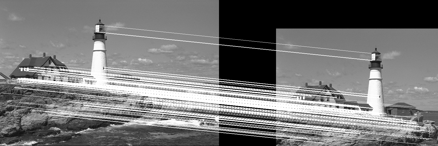
desc, ret_keypoints = create_descriptor(img, keypoints, brief_params)Results of using the BRIEF descriptor on a translated image.
ORB Keypoints and Descriptors
ORB (Oriented Fast and Rotated Brief) descriptor is similar to BRIEF but has an orientation detection mechanism. Apart from creating a descriptor, it also extracts keypoints over a gaussian pyramid using the FAST corners algorithm.
It can be used by calling the ORB constructor method.
orb_params = ORB([num_keypoints], [n_fast], [threshold], [harris_factor], [downsample], [levels], [sigma])
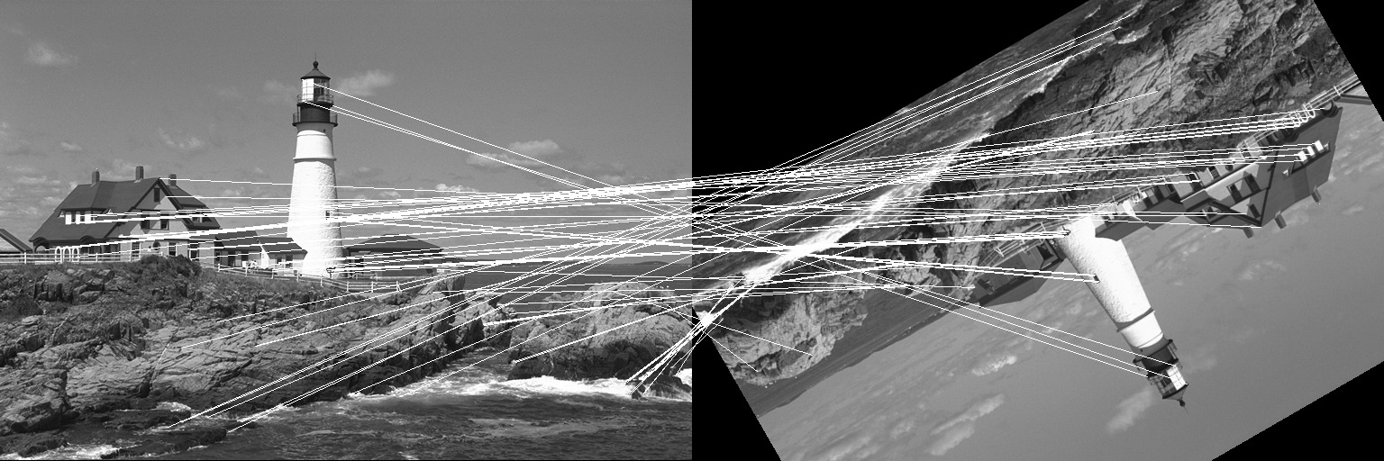
desc, ret_keypoints = create_descriptor(img, orb_params)Results of using the ORB descriptor on a translated and rotated image.
CENSURE Keypoints
Note : This PR is still open. The function needs more tests before it can be merged.
CENSURE (CENter SURround Extremas) keypoints are calculated using extremas at all scales and locations unlike SIFT or SURF which take extremas at each octave. To approximate the Laplacian operator, a bi-level (1 or -1) centre surround filter is used. Increasing size of the filter in each octave gives the result of the operator at different scales. Points of maxima and minima across the octaves are extracted as keypoints.
censure_params = CENSURE([smallest], [largest], [filter], [response_threshold], [line_threshold])
keypoints = extract_features(img, censure_params)
BRISK Descriptors
The BRISK (Binary Robust Invariant Scalable Keypoints) descriptor has a predefined sampling pattern as compared to BRIEF or ORB. Pixels are sampled over concentric rings.
The BRISK descriptor can be used by calling the BRISK constructor method to define the parameters and then using it with the create_descriptor API.
brisk_params = BRISK([pattern_scale])
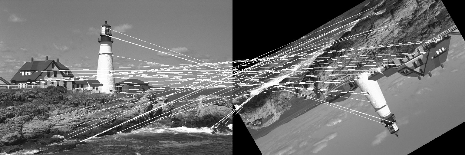
desc, ret_keypoints = create_descriptor(img, keypoints, brisk_params)Results of using the BRISK descriptor on a translated and rotated image.
FREAK Descriptors
The FREAK (Fast REtinA Keypoint) descriptor, similar to BRISK as a predefined sampling pattern. It uses a retinal sampling grid with more density of points near the centre with the density decreasing exponentially with distance from the centre.
The FREAK descriptor can be used by calling the FREAK constructor method to define the parameters and then using it with the create_descriptor API. Unlike BRISK, FREAK does not calculate the keypoints.
freak_params = FREAK([pattern_scale])
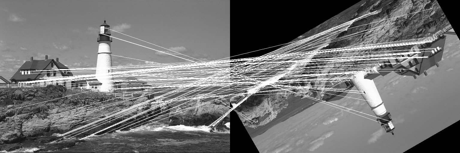
desc, ret_keypoints = create_descriptor(img, keypoints, freak_params)Results of using the FREAK descriptor on a translated and rotated image.
Drawing on Images
To help me understand how the feature detection algorithms were working, I needed a drawing library for Images in julia. Since it was already on the roadmap for JuliaImages, I developed proper APIs and created a new package, ImageDraw.jl.
Lines
The line and line! functions draw a line on the input image given the points p1, p2 as CartesianIndex{2} with the given color. Lines are drawn using the bresenham method by default. If anti-aliasing is required, the xiaolin_wu can be used.
img_with_line = line(img, p1, p2, color, method)
img_with_line = line(img, y0, x0, y1, x1, color, method)
To draw a line on the input image itself, use the line! function.
line!(img, p1, p2, color, method)Circles and Ellipses
The ellipse and ellipse! (similar use as line!) draw an ellipse on the input image given the center as a CartesianIndex{2} or as coordinates (y, x) using the specified color. If color is not specified, one(eltype(img)) is used.
img_with_ellipse = ellipse(img, center, radiusy, radiusx)
img_with_ellipse = ellipse(img, center, color, radiusy, radiusx)
img_with_ellipse = ellipse(img, y, x, radiusy, radiusx)
img_with_ellipse = ellipse(img, y, x, color, radiusy, radiusx)
Similarly the circle and its counterpart circle! functions may be used to draw circles.
img_with_circle = circle(img, center, radiusy, radiusx)
img_with_circle = circle(img, center, color, radiusy, radiusx)
img_with_circle = circle(img, y, x, radiusy, radiusx)
img_with_circle = circle(img, y, x, color, radiusy, radiusx)
Miscellaneous
Apart from the work discussed above, I also made minor contributions to two related packages, ColorVectorSpace.jl and ColorTypes.jl
Future Work
I am working on creating a set of tutorials on extracting features and using them to match images. The link to the tutorials can be found at the ImageFeatures.jl documentation website.